Return to MSc Portfolio.

Originally submitted as assessment material for the module:

 

Machine Learning and Predictive Analytics

 

Problem Identification

 

The problem to investigate is email spam filtering and the adaptability of a Machine Learning (ML) algorithm to correctly classify spam emails. Spam detection is critical to organisations and users across the globe, helping to improve cybersecurity and assist fraud prevention. In 2023 alone, an estimated 45.6% of all emails sent globally were identified as spam (Statista, 2024). Filtering spam from inboxes using ML is a perfect example of bringing theory into practice in the real-world.

 

In this paper, spam emails will refer to malicious emails (e.g. phishing) or other unsolicited email whose arrival in an inbox is likely to cause annoyance to a user. I set out to build a predictive model which can classify emails using frequency-based features, specifically experimenting with language-agnostic features.

 

Dataset Description and Analysis

 

This analysis uses the Spambase dataset, originally released in 1999 by Hopkins et al. It contains 4,601 instances with 57 features (Hopkins et al., 1999). To create the dataset, researchers collected spam emails provided by their internal postmaster at Hewlett-Packard Labs and other individuals, along with non-spam emails collected from personal emails. The dataset features were generated by exploring the frequency that terms appeared in an email. They also created features which measured the run-length of sequences of consecutive capital letters.

 

The dataset was compiled in 1999. As a result, spam habits and emails are likely to have changed in the decades since. This is known as Concept Drift, which Singhal et al. (2020) described as a scenario “…where the relation between the input data and the target variable changes over time…”. Whilst time has passed, I feel that the variety of features and number of instances available lend well to a simple language-agnostic experiment to detect spam.

 

After the dataset was imported, checks were performed for missing values. An additional check was conducted for any duplicate instances (emails). This would be possible since the authors noted the emails were sourced “…from our postmaster and individuals who had filed spam.” (Hopkins et al., 1999) and as such there could be overlap. This check resulted in the removal of 391 instances (emails) where a copy was already present, leaving 4,210 instances remaining. Duplicates were removed to prevent data leakage between training and testing sets.

 

A multivariate analysis will be conducted. This is justified since the dataset has multiple features available for analysis such as dollar signs, exclamation marks, and numbers.

 

Of the 57 available features I have selected the only 12 features which are numbers or symbols, as these fit my approach of being language agnostic. I rejected the feature word_freq_3d as this is mixed. Spam emails often rely on exaggerated visuals, such as the overuse of dollar signs or large monetary amounts. This approach is grounded in research. In a 2024 article, Longtchi et al. found a direct correlation between Attention Grabbing techniques (bold fonts, uppercase letters, highlighted text) and Visual Deception (replacing “vv” with “w”) in malicious emails (Longtchi et al., 2024).

 

The 12 features are listed in Table A, including examples of the first and last instances, along with the Target, Class.

 

Instance #	#0	#1	#2	#3	#4	#4205	#4206	#4207	#4208	#4209
word_freq_000	0	0.43	1.16	0	0	0	0	0	0	0
word_freq_650	0	0	0	0	0	0	0	0	0	0
word_freq_857	0	0	0	0	0	0	0	0	0	0
word_freq_415	0	0	0	0	0	0	0	0	0	0
word_freq_85	0	0	0	0	0	0	0	0	0	0
word_freq_1999	0	0.07	0	0	0	0	0	0	0	0
char_freq_;	0	0	0.01	0	0	0	0	0.102	0	0
char_freq_(	0	0.132	0.143	0.137	0.135	0.232	0	0.718	0.057	0
char_freq_[	0	0	0	0	0	0	0	0	0	0
char_freq_!	0.778	0.372	0.276	0.137	0.135	0	0.353	0	0	0.125
char_freq_$	0	0.18	0.184	0	0	0	0	0	0	0
char_freq_#	0	0.048	0.01	0	0	0	0	0	0	0
Class	1	1	1	1	1	0	0	0	0	0
Table A: Selected Features, showing the first and last instances in Spambase.

 

Algorithm Selection

 

The primary choice of algorithm for this task is LR. As a form of supervised learning, LR can be trained with past examples of spam, enabling classification of unseen examples. Pal (2021) writes in Cancer Research, Statistics, and Treatment (CRST) of how multivariate LR is a widely accepted form of ML for cancer diagnosis, which uses the past experience of patients to estimate an outcome by modelling previous data. Whilst this dataset is not predicting the outcome of cancer, it is following the same multivariate approach to create a binary classification (spam/not spam).

 

As well as classification, probabilities can be produced by LR, enabling custom thresholds to be set if required, as well as providing confidence levels e.g. “a 90% chance this email is spam”. LR is computationally efficient compared to other models, with a fast training and prediction speed, it also provides the ability to understand which features are having the most effect on predictions. There are risks of course, such as overfitting, or non-linearity within features. However, the input features are all numerical with linear relationships between them. For example, the frequency of the dollar sign appearing in an email, and whether it was classed as spam.

 

The model was implemented using Scikit-learn (Pedregosa et al., 2011). Prior to fitting the model, a Train/Test/Split was performed with 80% training, 20% testing, giving 3,368 and 842, respectively. The LR model was implemented using Scikit-learn’s LogisticRegressionCV function. This essentially allowed for various configurations to be tested, with the best model automatically selected. Features were scaled and a selection of regularisation values were provided. Cross-validation was set to five, to aid with the selection of the best model. The best model produced an accuracy score of 81.7%.

 

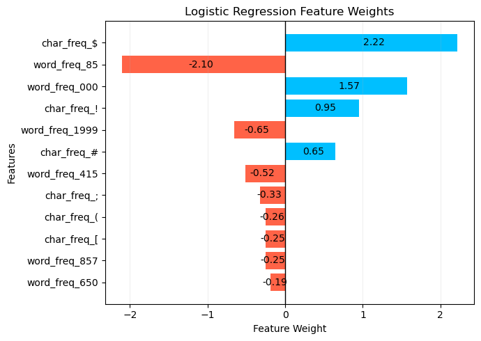
An advantage of LR as previously mentioned, is the high interpretability of the model. Feature coefficients, or weights, can be examined to determine which had more impact. Figure 1 shows the outcome of the 12 features. As might be expected, an email was more likely to be marked spam if it had a high use of dollar signs, multiple zeros, and exclamation marks.

 

Figure 1: Feature weighting from the Logistic Regression model.

 

Evaluation

 

Various metrics are available to interpret the performance of the model. As Bonaccorso notes (2018, p.184), “The performances of all classifiers must be measured using different approaches…” and as such we will consider a Receiver Operating Characteristic (ROC) plot, a Confusion Matrix, and Classification Metrics. For the purposes of this implementation the default classification score of 50% will remain, this is an experimental implementation based on language agnostic features. The default scoring will also enable easy comparison to an alternative model.

 

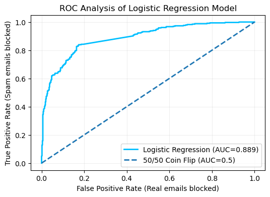
Initially let us explore a ROC plot shown in Figure 2. Broadly, the graph appears to be performing well, with an Area Under the Curve (AUC) score of 0.889 (3.d.p).  AUC scores range from 0.5 (no better than a coin flip) to 1.0 (a perfect score) and each graph should be taken in context to its application. Indeed, a study published in 2022 in The Lancet, considered AUC scores published in COVID-19 research material. Our score of 0.889 could have been graded anywhere from Fair to Excellent depending on institution (de Hond et al., 2022).

 

Figure 2: ROC Plot of the Logistic Regression model, with added 50/50 comparison.

 

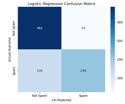
We can next visualise the model’s performance by implementing a Confusion Matrix, shown in Figure 3. Within our total test set of 842, the model correctly identified 206 and 482 emails as spam and not spam, respectively. There were 130 (15.4%) instances where spam emails evaded the model. 24 Emails (2.9%) were false positives and had this been a real email filter, may have been automatically deleted or moved to a spam folder. Considering that this is based only on the frequency of numbers and symbols, these are promising results.

 

Figure 3: Confusion Matrix breaking down the model’s performance over the test set.

 

Finally, we can consider performance metrics such as precision and recall. Table 2 shows the classification results over the test set of 842. Whilst the model had a high precision and was very accurate when it did detect spam (89.6%), it only managed to correctly locate 61.3% of spam instances. This is in line with the Confusion Matrix metrics of 130 false negatives. When predicting not spam it clearly performed better, isolating 95.3% of all instances, although its confidence had a lower precision at 78.8%, in line with the 24 false positives.

 

 

 

		Precision	Recall	F1
	Not Spam	78.8%	95.3%	86.2%
	Spam	89.6%	61.3%	72.8%
	Table 2: Classification results for Logistic Regression over the test set.

 

Overall, the LR model has fared well with only 12 features.

 

Comparative Analysis

 

An alternative model for classifying spam could be k-Nearest Neighbours (kNN), another form of supervised learning. A kNN model was implemented as a comparative exercise against LR. The same Train/Test/Split methodology was implemented with a common random variable ensuring the same training and test sets. Scikit-learn’s GridSearchCV capability was employed with an initial k-value as the square root of the training set, which was expanded either side to allow a range of values to be tested. Features were scaled with StandardScaler(), to help prevent higher values from skewing the distance calculations. The same scaler was used with the LR model. The grid search also tested Euclidean and Manhattan distances, cross-validation was set to five sets, as with LR.

 

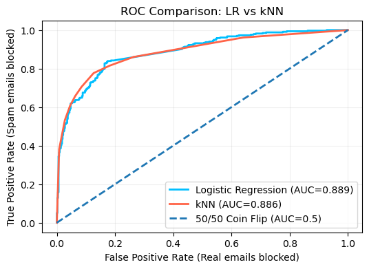
In comparison to LR, the kNN model achieved an accuracy score of 83.1%. A subtle improvement of 1.4% over LR. Although when calculating the AUC score, there was a slight decrease in score by 0.003, at 0.886. This is illustrated in Figure 4 which shows an ROC comparison between the two models, where LR comes out ahead.

 

Figure 4: ROC comparison between the Logistic Regression and kNN models.

 

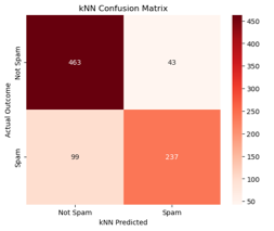
Figure 5 illustrates the kNN confusion matrix performance. The kNN model has managed to increase the true-positive spam detection whilst also reducing the number of false negatives. However, the false positive category has a notable increase to 43, whereas LR only marked 24 false positives. In the context of a spam filter where emails may be deleted or filtered from mailboxes, this is a notable decrease in performance.

 

Figure 5: Confusion Matrix showing the performance of kNN over the test set.

 

We can compare the classification metrics for both models side-by-side. Table 3 shows the consolidated F1 scores are higher for kNN which on paper would normally suggest a better performance, given also that the kNN model located 70.5% of the spam emails. However, as shown with the confusion matrix there was a noticeable drop in performance with real emails being misclassified as spam. On balance, a user is more likely to accept seeing the occasional spam email, than have their real mail hidden or deleted.

 

			Precision	Recall	F1
	Not Spam	LR	78.8%	95.3%	86.2%
		kNN	82.4%	91.5%	86.7%
	Spam	LR	89.6%	61.3%	72.8%
		kNN	84.6%	70.5%	76.9%
Table 3: Classification comparison between Logistic Regression and kNN over the test set.

 

As a lazy-learning methodology, kNN models can accept multiple features such as those present in the current dataset, and whilst a kNN model can be trained and deployed to detect spam email it does have some distinct disadvantages over LR. These include a lower interpretability at a feature level; it is difficult to determine which features are having the most influence over the model. There is also the computational cost to consider. Cunningham and Delany (2022) explained that since all the work is done at runtime, a kNN model can have poor runtime performance if a large training set is used. This is important considering that a spam filter may have to consider millions of emails at any given moment.

 

Based on the results of the two models and a comparison of strengths and limitations, kNN can be rejected as a primary choice for classifying spam emails. Whilst it has some potential, the inability to examine which features are having the most impact, alongside the lower prediction speed, make kNN unsuitable at scale.

 

 

Conclusion

 

An LR model based solely on features containing numbers or symbols, has at least some real-world potential and could be explored further at scale. The implementation of the model allowed 95.3% of real emails through its filter, although with a disappointing catchment of only 61.3% of spam. However, this is before any advanced feature engineering and adjustments to coefficients. A comparative implementation of a kNN model only allowed 91.5% of real emails through.

 

This is not to say that LR is the very best approach. Recently in an experiment by Zavrak and Yilmaz (2023), analysing the performance of Convolutional Neural Networks (CNN) for spam detection, a CNN approach outperformed existing ML models in several areas. Ultimately, on the balance of accuracy, interpretability, and computational cost, an LR model would be suitable for a real-world implementation of a language agnostic spam-filter.

 

 

 

Word count (excluding references): 2,176

 

 

Bibliography

 

Bonaccorso, G. (2018) Machine learning algorithms: popular algorithms for data science and machine learning. Second edition. Birmingham; Packt Publishing.

 

Cunningham, P., Delany, S. J. (2022) k-Nearest Neighbour Classifiers - A Tutorial. ACM computing surveys [online] 54(6), pp. 1 [Accessed 18 January 2026]

 

de Hond, Anne A H et al. (2022) Interpreting area under the receiver operating characteristic curve. The Lancet Digital Health [online] 4(12), pp. 853-855. [Accessed 15 January 2026]

 

Hopkins, M., Reeber, E., Forman, G., Suermondt, J. (1999). Spambase, UCI Machine Learning Repository [online]. Available from: http://archive.ics.uci.edu/dataset/94/spambase [Accessed 11 January 2026]

 

Longtchi, T. et al. (2024) Quantifying Psychological Sophistication of Malicious Emails. IEEE access. [Online] 12, pp. 187512-187535. [Accessed 17 January 2026]

 

Pal, K. (2021) Logistic regression: A simple primer. Cancer Research, Statistics, and Treatment [online]. 4(3), pp. 551-554. [Accessed 18 January 2026]

 

Pedregosa et al. (2011) Scikit-learn: Machine Learning in Python. Journal of Machine Learning Research [online]. JMLR 12, pp. 2825-2830. [Accessed 11 January 2026]

 

Singhal, S., Chawla, U., Shorey, R., ed. (2020) Machine Learning & Concept Drift based Approach for Malicious Website Detection, 2020 International Conference on COMmunication Systems & NETworkS (COMSNETS), Bengaluru, India, 7-11 January 2020. IEEE [online]. Available from: https://ieeexplore-ieee-org.uwe.idm.oclc.org/document/9027485 [Accessed 18 January 2026]

 

Statista (2024) Global spam volume as percentage of total e-mail traffic from 2011 to 2023. Available from: https://www.statista.com/statistics/420400/spam-email-traffic-share-annual/ [Accessed 14 January 2026]

 

Zavrak, S., Yilmaz, S. (2023) Email spam detection using hierarchical attention hybrid deep learning method. Expert systems with applications [Online] 233(120977) [Accessed 18 January 2026]